◦
suggested reads:
cryptography, security, and random thoughts
Hey! I'm David, cofounder of zkSecurity, advisor at Archetype, and author of the Real-World Cryptography book. I was previously a cryptography architect of Mina at O(1) Labs, the security lead for Libra/Diem at Facebook, and a security engineer at the Cryptography Services of NCC Group. Welcome to my blog about cryptography, security, and other related topics.
Any bleeding-edge field has trouble agreeing on terms, and only with time some terms end up stabilizing and standardizing themselves. Some of these terms are a bit weird in the zero-knowledge proof field: we talk about SNARKs and SNARGs and zk-SNARKs and STARKs and so on.
It all started from a clever pun “succinct non-interactive argument of knowledge” and ended up with weird consequences as not every new scheme was deemed “succinct”. So much so that naming branched (STARKs are “scalable” and not “succinct”) or some schemes can’t even be called anything. This is mostly because succinct not only means really small proofs, but also really small verifier running time.
If we were to classify verifier running time between the different schemes it usually goes like this:
Using the almost-standardized categorization, only the first one can be called a SNARK, the second one is usually called a STARK, and I’m not even sure how we call the third one, a NARK?
But does it really make sense to reserve SNARK to the first scheme? It turns out people are using all three schemes because they are all dope and fast(er) than running the program by yourself. Since SNARK has become the main term for general-purpose zero-knowledge proofs, then let’s just use that!
I’m not the only one that wants to call STARKs and bulletproofs SNARKs, Justin Thaler also makes that point here:
the “right” definition of succinct should capture any protocol with qualitatively interesting verification costs – and by “interesting,” I mean anything with proof size and verifier time that is smaller than the associated costs of the trivial proof system. By “trivial proof system,” I mean the one in which the prover sends the whole witness to the verifier, who checks it directly for correctness
On the A16Z’s blog, Sreeram Kannan and Soubhik Deb wrote a great article on the cryptoeconomics of slashing.
If you didn’t know, slashing is the act of punishing malicious validators in BFT consensus protocols by taking away tokens. Often tokens that were deposited and locked by the validators themselves in order to participate in the consensus protocol. Perhaps the first time that this concept of slashing appeared was in Tendermint? But I’m not sure.
In the article they make the point that BFT consensus protocols need slashing, and are less secure without it. This is an interesting claim as there’s a number of BFT consensus protocols that are running without slashing (perhaps a majority of them?)
Slashing is mostly applied to safety violations (a fork of the state of the network) that can be proved. This is often done by witnessing two conflicting messages being signed by the same node in the protocol (often called equivocation). Any “forking attack” that want to be successful will require a threshold (usually a third) of the nodes signing conflicting messages.
Slashing only affects nodes that still have stake in the system, meaning that forking old history to target a node that’s catching up (without a checkpoint) doesn’t get affected by slashing (what we call long-range attacks). The post argues that we need to separate the cost-of-corruption from the profit-from-corruption and seem to only assume that the cost-of-corruption is always the full stake of all attackers, in which case this analysis only makes sense in attacks aiming at forking the tip/head of the blockchain.
The post present a new model, the Corruption-Analysis model, in order to analyze slashing. They accompany the model with the following table that showcases the different outcomes of an attack in a protocol that does not have slashing:
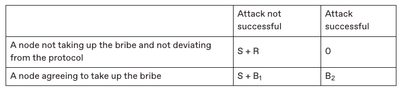
Briefly, it shows that (in the bottom-left corner) failed attacks don’t really have a cost as attackers keep their stake (S) and potentially get paid (B1) to do the attack. On the other hand it shows that (in the top-right corner) people will likely punish everyone in case of an attack by mass selling and taking the token price down to (an implied feature they call token toxicity).
On the other hand, this is the table they show once slashing is integrated:
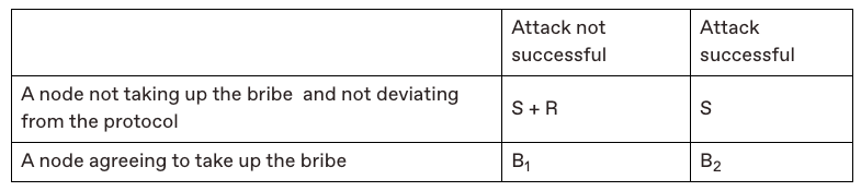
As one can see, the bottom-left corner and the top-right corner have changed: a failed attack now has a cost, and a successful attack almost doesn’t have one anymore. Showing that slashing is strictly better than not slashing.
While this analysis is great to read, I’m not sure I fully agree with it. First, where did the “token toxicity” go in the case of a successful attack? I would argue that a successful attack would impact the protocol in similar ways. Perhaps not as intensely, as as soon as the attack is detected the attackers would lose their stake and not be able to perform another attack, but still this would show that the economic security of the network is not good enough and people would most likely lose their trust in the token.
Second, is the case where the attack was not successful really a net improvement? My view is that failed attacks generally happen due to accidents rather than legitimate attempts, as an attacker would most likely succeed if they had enough to perform an attack. And indeed, I believe all of the slashing events we’ve seen were all accidents, and no successful BFT attacks was ever witnessed (slashing or no slashing). (That being said, there are cases where an attacker might have difficulties properly isolating a victim’s node, in which case it might be harder to always be successful at performing the attack. This really depends on the protocol and on the power of the adversary.)
In addition, attacks are all different. The question of who is targeted matters: if the victim reacts, how long does it take them to punish the attackers and publish the equivocation proofs? Does the protocol has a long-enough unstaking period to give the victim time to punish them? And if a third of the network is Byzantine, can they prevent the slashing from happening anyway by censoring transactions or something? Or worst case, can they kill the liveness of the network instead of getting slashed, punishing everyone and not just them (up until a hard fork occurs)?
Food for thought, but this shows that slashing is still quite hard to model. After all, it’s a heuristic, and not a mechanism that you will find in any BFT protocol whitepaper. As such, it is part of the overall economic security of the deployed protocol and has to be measured via both its upsides and downsides.
I think a lot about how to express concepts and find good abstractions to communicate about proof systems. With good abstractions it’s much easier to explain how proof systems work and how they differ as they then become more or less lego-constructions put up from the same building blocks.
For example, you can sort of make these generalization and explain most modern general-purpose ZKP systems with them:
Knowing these 4-5 points will get you a very long way. For example, you should be able to quickly understand how STARKs work.
Having said that, I more recently noticed another pattern that is used all over the place by all these proof systems, yet is never really abstracted away, the interactive arithmetization pattern (for lack of a better name). Using this concept, you can pretty much see AIR, Plonkish, and a number of protocols in the same way: they’re basically constraint systems that are iteratively built using challenges from a verifier.
Thinking about it this way, the difference between STARK’s AIR and Plonks’ plonkish arithmetization is now that one (Plonk) has fixed columns that can be preprocessed and the other doesn’t. The permutation of Plonk is now nothing special, the write-once memory of Cairo is nothing special as well, they’re both interactive arithmetizations.
Let’s look at plonk as a table, where the left table is the one that is fixed at compilation time, and the right one is the execution trace that is computed at runtime when a prover runs the program it wants to prove:

One can see the permutation argument of plonk as an extra circuit, that requires 1) the first circuit to be ran and 2) a challenge from the verifier, in order to be secure.
As a diagram, it would look like this:

Now, one could see the write-once memory primitive of Cairo in the same way (which I explained here), or the lookup arguments of a number of proof systems in the same way.
For example, the log-derivative lookup argument used in protostar (and in most protocols nowadays) looks like this. Notice that:

As such, the point I really want to make is that a number of ZKP primitives and interaction steps can be seen as an interactive process to construct a super constraint system from a number of successive constraint system iterated on top of each other. Where constraint system means “optionally some new fixed columns, some new runtime columns, and some constraints on all the tables including previous tables”. That’s it.
Perhaps we should call these iterative constraint systems.
In this episode, David Wong introduces Ethereum and explains its account-based model and the concept of smart contracts. He compares Ethereum to Bitcoin and highlights the advantages of Ethereum’s more expressive programming capabilities. He also discusses the execution of transactions and the role of the Ethereum network in maintaining the state of smart contracts.
In this episode, David Wong interviews Kevin Hurley and Alex Akselrod to discuss layer 2 solutions on Bitcoin. They explain that layer 2 (L2) is a scalability solution that sits on top of the Bitcoin blockchain and adds additional functionality and programmability. They discuss the history of L2s, mentioning Namecoin and colored coins as early examples. They also explore the distinction between L2s and sidechains, with L2s typically allowing for unilateral exits and sidechains relying on federations or merge mining. They mention projects like Blockstream, Stacks, and Rootstock as examples of L2s or sidechains on Bitcoin. The conversation explores the concept of multi-signature (multi-sig) and its role in layer 2 (L2) solutions like Liquid. It also delves into the workings of the Lightning Network, which enables instant and low-cost transactions on Bitcoin. The Lightning Network operates through payment channels, where users can push ‘beads’ (Satoshi’s) back and forth. The conversation also touches on the challenges of centralization in Lightning Network and the role of LightSpark in making Lightning more accessible and user-friendly.
Guillermo tricked me into recording some whiteboard sessions to introduce the concept of multi-party computations along with some of the schemes and tricks used to build them. I had fun recording these, hope you have fun watching :)
As I explained here a while back, checking polynomial identities (some left-hand side is equal to some right-hand side) when polynomials are hidden using polynomial commitment schemes, gets harder and harder with multiplications. This is why we use pairings, and this is why sometimes we “linearize” our identities. If you didn’t get what I just said, great! Because this is exactly what I’ll explain in this post.
First, let me say that there’s typically two types of “nice” polynomial commitment schemes that people use with elliptic curves: Pedersen commitments and KZG commitments.
Pedersen commitments are basically hidden random linear combinations of the coefficients of a polynomial. That is, if your polynomial is your commitment will look like for some base point and unknown random values . This is both good and bad: since we have access to the coefficients we can try to use them to evaluate a polynomial from its commitment, but since it’s a random linear combination of them things can get ugly.
On the other hand, KZG commitments can be seen as hidden evaluations of your polynomials. For the same polynomial as above, a KZG commitment of would look like for some unknown random point . Not knowing here is much harder than not knowing the values in Pedersen commitments, and this is why KZG usually requires a trusted setup whereas Pedersen doesn’t.
In the rest of this post we’ll use KZG commitments to prove identities.
Let’s use to mean “commitment of the polynomial “, then you can easily check that knowing only the commitments to and by checking that or . This is because of the Schwartz-Zippel (S-Z) lemma which tells us that checking this identity at a random point is convincing with high-enough probability.
When multiplication with scalars is required, then things are fine. As you can do to obtain , checking that is as simple as checking that .
This post is about explaining how pairing helps us when we want to check an identity that involves multiplying and together.
It turns out that elliptic curve pairings allow us to perform a single multiplication. Meaning that once things get multiplied, they move to a different planet where things can only get added together and compared. No more multiplications.
Pairings give you this function which allows you to move things in the exponent like this: . Where, remember, is the multiplication of the two polynomials evaluated at a random point: .
As such, if you wanted to check something like this for example: with commitments only, you could check the following pairings:
By the way, the left argument and the right argument of a pairing are often in different groups for “reasons”. So we usually write things like this:
And so it is important to have commitments in the right groups if you want to be able to construct your polynomial identity check.
But what if you want to check something like ? Are we doomed?
We’re not! One insight that plonk brought to me (which potentially came from older papers, I don’t know, I’m not an academic, leave me alone), is that you can reduce the number of multiplication with “this one simple trick”. Let me explain…
A typical scenario includes you wanting to check an identity like this one:
and you have KZG commitments to all three polynomials . (So in other words, hidden evaluations of these polynomials at the same unknown random point )
You can’t compute the commitment of the left-hand side because you can’t perform the multiplication of the three commitments.
The trick is to evaluate (using KZG) the previous identity at a different point, let’s say , and pre-evaluate (using KZG as well) as many polynomials as you can to to reduce the number of multiplications down to 0.
Note: that is, if we want to check that is true, and we want to use S-Z to do that at some point , then we can pre-evaluate (or ) and check the following identity at some point instead.
More precisely, we’ll choose to pre-evaluate and , for example. This means that we’ll have to produce a quotient polynomial and such that:
which means that the verifier will have to perform the following two pairings (after having been sent the evaluation and in the clear):
Then, they’ll be able to check the first identity at and use and in place of the commitments and . The verifier check will look like the following pairing (after receiving a commitment from the prover):
which proves using KZG that (which proves that the identity checks out with high probability thanks to S-Z).
In the previous explanation, we actually perform 3 KZG evaluation proofs instead of one:
Pairings can be aggregated by simply creating a random linear combinations of the pairings. That is, with some random values we can aggregate the checks where the left-hand side is:
and the right-hand side is:
I’ve recorded a video on how the plonk permutation works here, but I thought I would write a more incremental explanation about it for those who want MOAR! If things don’t make sense in this explanation, I’m happy to dig into specifics in more detail, just ask in the comments! Don’t forget your companion eprint paper.
Suppose that you have two ordered sets of values and , and that you want to check that they contain the same values. That is, you want to check that there exists a permutation of the elements of (or ) such that the multisets (sets where some values can repeat) are the same, but you don’t care about which permutation exactly gets you there. You’re willing to accept ANY permutation.
For example, it could be that re-ordering as gives us exactly .
One way to do perform our multiset equality check is to compare the product of elements on both sides:
If the two sets contain the same values then our identity checks out. But the reverse is not true, and thus this scheme is not secure.
Can you see why?
For example, and are obviously different multisets, yet the product of their elements will match!
What we can do to fix this issue is to encode the values of each lists as roots of two polynomials:
These two polynomials are equal if they have the same roots with the same multiplicities (meaning that if a root repeats, it must repeat the same number of times).
Now is time to use the Schwartz-Zippel lemma to optimize the comparison of polynomials! Our lemma tells us that if two polynomials are equal, then they are equal on all points, but if two polynomials are not equal, then they differ on MOST points.
So one easy way to check that they match with high probability is to sample a random evaluation point, let’s say some random . Then evaluate both polynomials at that random point to see if their evaluations match:
The previous check is not useful for wiring different cells within some execution trace. There is no specific “permutation” being enforced. So we can’t use it as in in plonk to implement our copy constraints.
To enforce a permutation, we can compare tuples of elements instead! For example, let’s say we want to enforce that must be re-ordered using the permutation in cycle notation. Then we would try to do the following identity check:
Here, we are enforcing that is equal to , and that is equal to , etc. This allows us to re-order the elements of :
But how can we encode our tuples into the polynomials we’ve seen previously? The trick is to use a random linear combination! (And that is often the answer in a bunch of ZK protocol.)
So if we want to encode in an equation, for example, we write for some random value .
Note: The rationale behind this idea is still due to Schwartz-Zippel: if you have two tuples and you know that the polynomials is the same as the polynomial if and , or if you have . If is chosen at random, the probability that it is exactly that value is with the size of your sampling domain (i.e. the size of your field) which is highly unlikely.
So now we can encode the previous lists of tuples as these polynomials:
And then reduce both polynomials to a single value by sampling random values for and . Which gives us:
If these two values match, with overwhelming probability we have that the two polynomials match and thus our permutation of matches .
Let’s now see how we can use the (optimized) checks we’ve learn previously in plonk. We will first learn how to wire cells of a single execution trace column, and in the next section we will expand this to three columns (as vanilla Plonk uses three columns).
Take some moment to think about how can we use the previous stuff.
The answer is to see the execution trace as your list , and then see if it is equal to a fixed permutation of it (). Note that this permutation is decided when you write your circuit, and precomputed into the verifier key in Plonk.
Remember that the formula we’re trying to check is the following for some random and , and for some permutation function that we defined:
To enforce the previous check, we will write a mini-circuit (yes an actual circuit!) which will progressively accumulate the result of dividing the left-hand side with the right-hand side. This circuit only requires one variable/register we’ll call (and so it will add a new column in our execution trace) which will start with the initial value 1 and will end with the following value:
Let’s rewrite it using only the first wire/column of Plonk, and using our generator as index in our tuples (because this is how we handily index things in Plonk):
We can then constrain the last value to be equal to 1, which will enforce that the two polynomials encoding our list of value and its permutation are equal (with overwhelming probability).
In plonk, a gate can only access variables/registers from the same row. So we will use the following extra gate (reordering the previous equation, as we can’t divide in a circuit) throughout the circuit:
Now, how do we encode this gate in the circuit? The astute eye will have noticed that we are using a cell of the next row () which we haven’t done in Plonk so far.
Enforcing things across rows is actually possible in plonk because we encode our polynomials in a multiplicative subgroup of our field! Due to this, we can reach for the next value(s) by multiplying an evaluation point with the subgroup’s generator.
That is, values are encoded in our polynomials at evaluation points , and so multiplying an evaluation point by (the generator) brings you to the next cell in an execution trace.
As such, the verifier will later try to enforce that the following identity checks out in the multiplicative subgroup:
Note: This concept was generalized in turboplonk, and is used extensively in the AIR arithmetization (used by STARKs). This is also the reason why in Plonk we have to evaluate the polynomial at .
There will also be two additional gates: one that checks that the initial value is 1, and one that check that the last value is 1, both applied only to their respective rows. One trick that Plonk uses is that the last value is actually obtained in the last row. As last_value + 1 = 0 in our multiplicative subgroup, we have that is constrained automatically. As such, checking that is enough.
You can see these two gates added to the vanilla plonk gate in the computation of the quotient polynomial in plonk. Take a look at this screenshot of the round 3 of the protocol, and squint really hard to ignore the division by , the powers of being used to aggregate the different gate checks, and the fact that and (the other wires/columns) are used:

The first line in the computation of is the vanilla plonk gate (that allows you to do multiplication and addition); the last line constrains that the first value of is ; and the other lines encode the permutation gate as I described (again, if you ignore the terms involving and ).
There’s something worthy of note: the extra execution trace column contains values that use other execution trace columns. For this reason, the other execution trace columns must be fixed BEFORE anything is done with the permutation column .
In Plonk, this is done by waiting for the prover to send commitments of , , and to the verifier, before producing the random challenges and that will be used by the prover to produce the values of .
The previous check only works within the cells of a single execution trace, how does Plonk generalizes this to several execution trace columns?
Remember: we indexed our first execution trace column with the values of our circuit domain (that multiplicative subgroup), we simply have to find a way to index the other columns with distinct values.
A coset is simply a set that is the same size as another set, but that is completely disjoint from that set. Handily, a coset is also defined as something that’s very easy to compute if you know a subgroup: just multiply it with some element .
Since we want a similar-but-different set from the elements of our multiplicative subgroup, we can use cosets!
Plonk produces the values and (which can be the values and , for example), which when multiplied with the values of our multiplicative subgroup () produces a different set of the same size. It’s not a subgroup anymore, but who cares!
We now have to create three different permutations, one for each set, and each permutation can point to the index of any of the sets.
Spent some time to write a challenge focused on GKR (the proof system) on top of the gnark framework (which is used to write ZK circuits in Golang).
It was a lot of fun and I hope that some people are inspired to try to break it :)
We’re using the challenge to hire people who are interested in doing security work in the ZK space, so if that interests you, or if you purely want a new challenge, try it out here: https://github.com/zksecurity/zkBank
And of course, since this is an active wargame please do not release your own solution or write up!